The notes for this course began from a series originally
written by Tim Ng, with extensions by
David Cash and
Robert Rand. I have modified them to follow our course.
Connectedness
What does it mean if there's a walk between two vertices? Practically
speaking, it means that we can reach one from the other. This idea leads to
the following definition.
A graph $G$ is connected if it
contains a path between every pair of vertices.
The graphs that we've seen so far have mostly been connected. However,
we're not guaranteed to work with connected graphs, especially in real-world
applications. In fact, we may want to test the connectedness of a graph. For
that, we'll need to talk about the parts of a graph that are connected.
A (connected) component of a graph
$G = (V,E)$ is a maximal connected subgraph $G$. In other words, it is a
connected subgraph that is not a proper subgraph of another connected
subgraph of $G$.
The maximality condition means that components are always induced
subgraphs: If not, then adding missing edges will give a larger subgraph.
Consider the following graph.
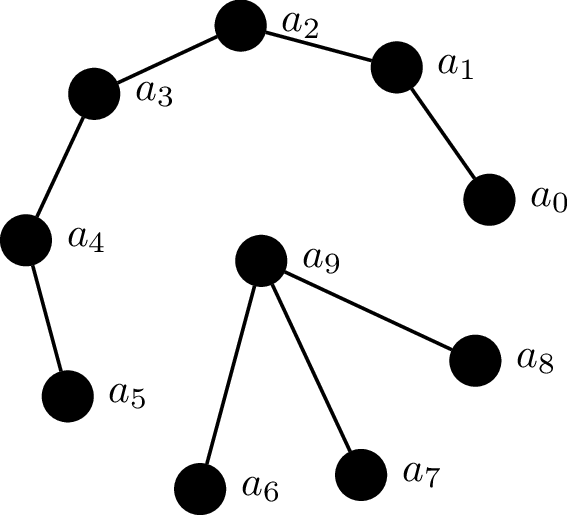
This graph has two components, the subgraphs induced by $a_0,\dots, a_5$
and $a_6,\dots,a_9$. No other can be considered a connected component since
they would either be not connected or a proper subgraph of one of the two
connected components we identified.
Every vertex belongs to exactly one component.
Consequently, the components of a graph partition its vertices.
Every vertex is contained in a connected component: The subgraph
consisting of only $v$ is connected trivially, and this subgraph is either
maximal or contained in a larger connected subgraph.
Now suppose that a vertex $u$ is in two distinct components $C_1, C_2$.
We will
show that $C_1 = C_2$. Let $v$ be a vertex of $C_1$ and $w$ be a vertex of
$C_2$. There there is a path from $u$ to $v$, and a path from $v$ to $w$. By
Theorem 10.14, there is a path from $v$ to $w$. Therefore we can add
$w$ to $C_1$ and still have a connected component. Since $C_1$ is maximal,
it must contain $w$. This shows that $C_1$ and contains every vertex of
$C_2$, and the same argument shows the reverse. Since $C_1$ and $C_2$ are
induced subgraphs on the same vertices, they are equal.
Bridges
Another question related to connectivity that we can ask is how fragile
the graph is. For instance, if we imagine some sort of network (computer,
transportation, social, etc.), this is the same as asking where the points
of failure are in our network. Which edges do we need to take out to
disconnect our graph?
We say an edge $e=uv$ is a bridge
if every path from $u$ to $v$ includes $e$.
Equivalently, $e=uv$ is a bridge if the graph $G - e$ (i.e. $G$ with $e$
deleted) has no path from $u$ to $v$.
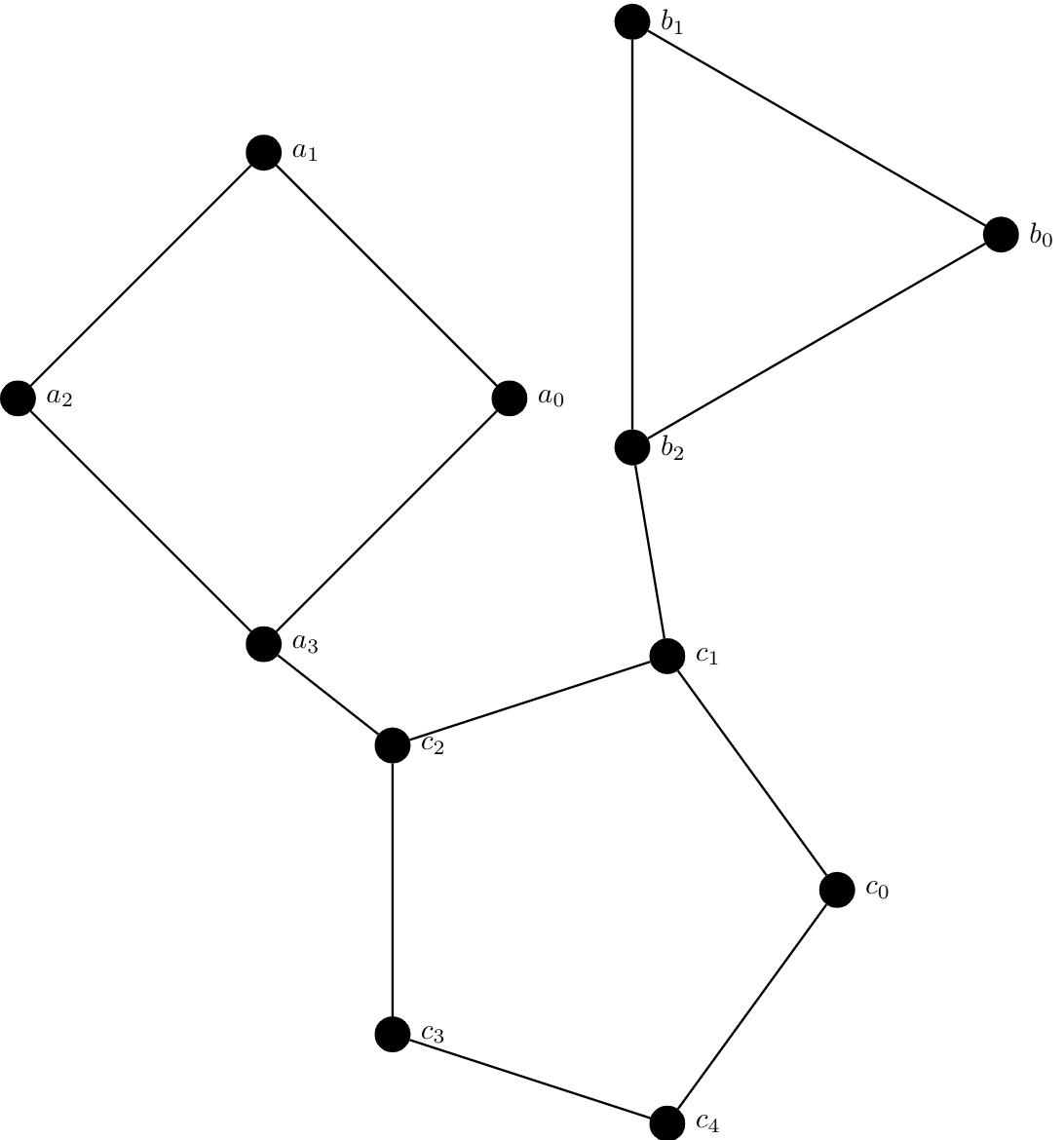
Consider the following graph $G$. There are two
visually-obvious
bridges here: $a_3c_2$ and $b_2c_1$.
Bridges have a simple and interesting characterization: They are
the edges that do not lie on any cycle.
Let $G$ be a graph. An edge $e$ of $G$ is a bridge if
and only if it is not contained in any cycle of $G$.
This theorem has the propositional form $p \leftrightarrow \neg q$ ($p$
is "$e$ is a bridge" and $q$ is "$e$ lies on a cycle"). We will prove it by
showing $\neg p \rightarrow q$ and $q \rightarrow \neg p$, which you can
check is logically equivalent.
For the "$q \rightarrow \neg p$" part, assume that $e = uv$ lies on a
cycle. Then there is a path $P$ in $G-e$ from $u$ to $v$: take the rest of
the cycle except for $e$. Thus $e$ is not a bridge.
For the "$\neg p \rightarrow q$" part, suppose that $e=uv$ is not a
bridge. Then $G-e$ contains a path from $u$ to $v$ that does not use
$e$. Adding $e$ to this path forms a cycle.
Trees
This part is about a special and familiar class of graphs called
trees. We used trees informally as a counting method in
combinatorics, and you've likely done some programming with trees. In those
cases the trees are usually rooted and drawn growing down from the
root (like in a family tree or organizational chart). Our treatment will be
more general, in that we won't designate a root. For example, the following
are both trees in this lecture:
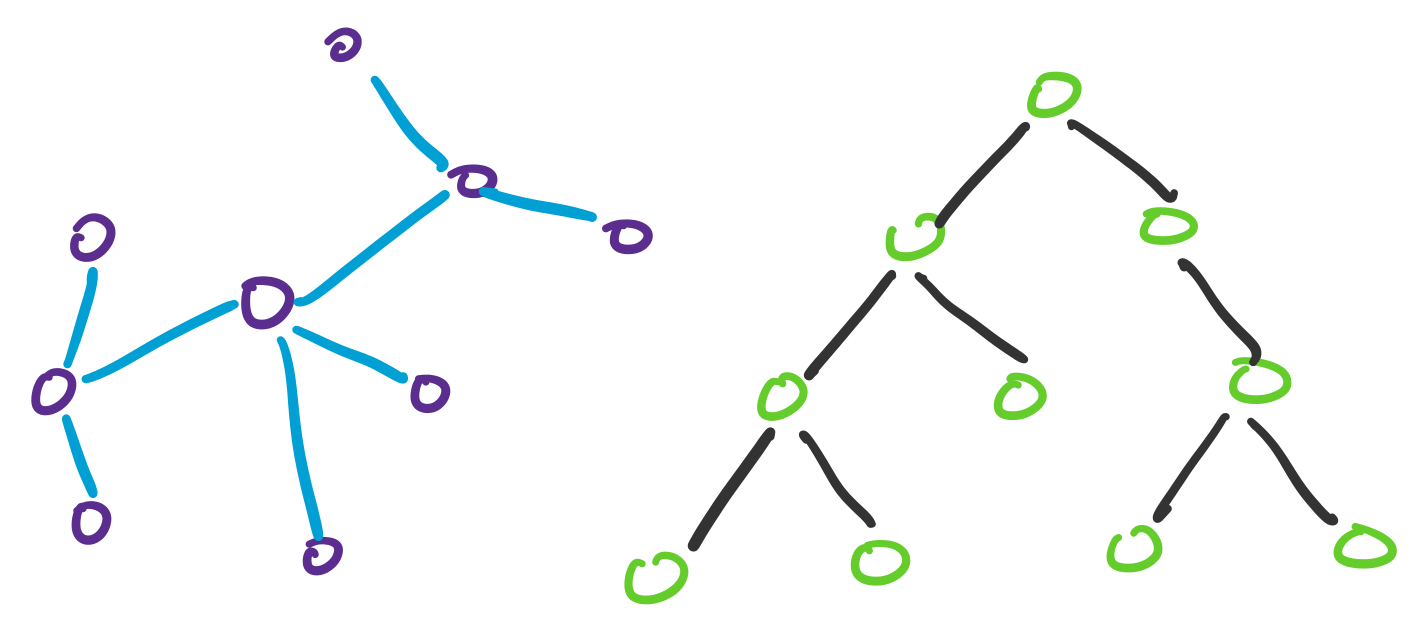
Here's the general, non-rooted, definition that we will use:
A graph $G$ is a tree if $G$ is
connected and contains no cycles. A graph $G$ with no cycles is a
forest.
Note that the definition of a tree is quite simple, but it has a clear
connection with our discussion of bridges and connectivity. Since a tree has
no cycles, this means that every edge in a tree is a bridge. In other words,
removing any edge in the graph will disconnect it.
The following are all equivalent:
- The graph $T$ is a tree.
- There is a unique path between any two vertices of $T$.
- The graph $T$ is connected and every edge is a bridge.
For this type of theorem, we need to prove that each condition is
equivalent. There are $\binom{3}{2}=3$ pairwise relationships being asserted,
which results in $3 \cdot 2=6$ implications that we'd need to prove,
but we don't need to do all of that work. Instead we'll prove a cycle
of implications $1. \implies 2. \implies 3. \implies 1.$, and this will
establish all of the pairwise implications.
$(1. \implies 2.)$ Suppose $T$ is a tree. Then $T$ is connected, and
hence there is at least one path between every pair of vertices. There is
only one distinct path between any pair of vertices because otherwise
Theorem 22.4 would imply $T$ contains a cycle and hence is not a tree.
$(2. \implies 3.)$ Suppose there is a unique path between any pair of
vertices in $T$. Then $T$ is connected. Let $e=uv$ be an edge of $T$. The
only path from $u$ to $v$ is the edge $e$, so $T-e$ does not contain a path
from $u$ to $v$. This shows that $e$ is a bridge.
$(3. \implies 1.)$ Suppose that $T$ is connected and every edge is a
bridge. By Theorem 11.6, no edge lies on a cycle. This shows there are
no cycles in $T$.
We next prove a structural theorem that is very useful for working with
trees: They have leaves. For proofs, having leaves allows us to
do induction on trees cleanly.
A vertex $v$ is called a leaf if
$d(v)=1$.
Any tree with two or more vertices contains a
leaf.
Let $P$ be the longest path in a given tree. Since $G$ contains at least
two vertices, this path has at least one edge. Let $v_0,\ldots,v_k$ be its
vertices in order. Then $d(v_k)\geq 1$. Suppose there is another edge
$v_ku$ ($u\neq v_{k-1}$) in $T$ incident to $v_k$. We can't have $u \in
\{v_0,\ldots,v_{k-2}$ because this edge would create a cycle. We also
can't have $u$ be a vertex outside the path, because then we could
extend $P$ to a longer path, a contradiction.
Here is a nice application of this.
A tree $T$ with $n\geq 1$ vertices has exactly $n-1$
edges.
We will show this by induction on $n$.
Base case. We have $n = 1$, and therefore, our graph
contains $0 = 1 - 1$ edges, so our statement holds.
Inductive case. Let $n \geq 1$ be arbitrary and assume
that every tree $T'$ with $n$ vertices has $n-1$ edges. Now, consider a tree
$T = (V,E)$ with $n+1$ vertices. By the previous theorem $T$ contains a leaf
$v$. Let $T' = T-v$ be the graph with $v$ and its edge deleted. Then $T'$ is
a still a tree (check why!), and it has $n$ vertices, so by induction $T'$
has $n-1$ edges. Since we removed one edge to form $T'$, $T$ has $(n-1)+1 =
n$ edges. This completes the induction.
Spanning Trees
We can apply the idea of a tree as a minimally connected graph to say
something about connectivity in graphs in general. One clear application is
finding a minimal connected subgraph of the graph such that every vertex is
connected. One can see how this might be useful in something like road network
where you're trying to figure out what the most important roads to clear after
a snowfall are.
A spanning subgraph which is also a tree is called
a spanning tree.
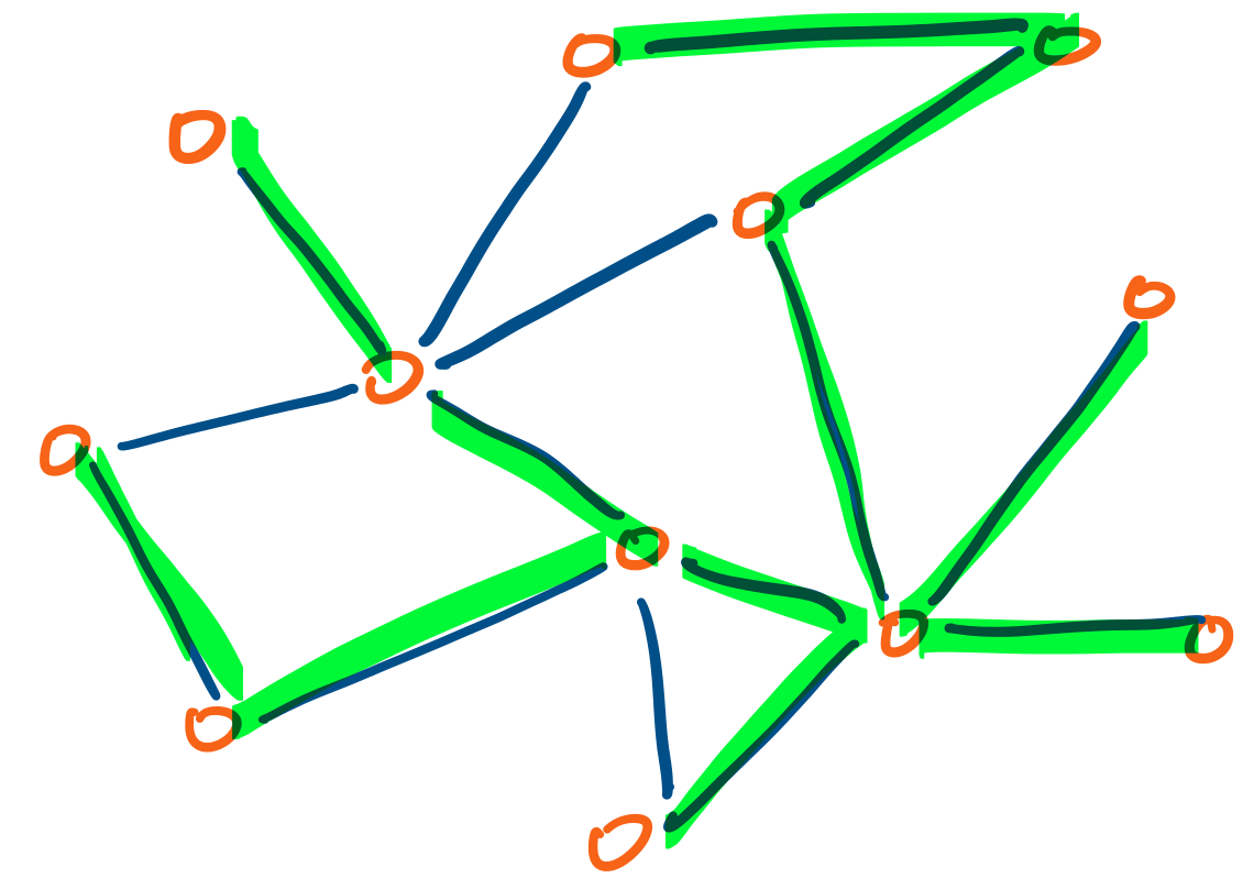
Here is a graph, with one possible spanning tree
highlighted.
A graph $G$ is connected if and only if it has a
spanning tree.
Suppose $G$ has a spanning tree $T$. Then there exists a path between
every pair of vertices in $T$ and therefore, there exists a path between
every pair of vertices in $G$. Then by definition, $G$ is connected.
Now, suppose $G$ is connected. Since it contains at least one connected
spanning subgraph (i.e., itself), we can consider the connected spanning
subgraph $H$ of $G$ with the minimal number of edges. If $H$ contained a
cycle, then we could remove an edge from this cycle, and get a smaller
connected spanning subgraph.
Therefore, $H$ contains no cycles and since $H$ is connected,
it is a tree.
Two Explorations
We'll end this class by presenting two explorations about trees that push
the limits of what we've learned in this class. They are also both peeks
into the kind of work that what we've done in this class leads to. The first is a sneak
peek of Algorithms (CMSC 272), and the second is a sneak peek into more advanced
techniques in graph theory. Both are just beyond the scope of this course.
Greedy Algorithm for Spanning Trees
The proof of Theorem 11.14 is called "non-constructive": It convinces
us that a spanning tree exists, but doesn't really say how to find one.
We'll now do a different proof that does.
We haven't discussed how graphs are implemented in algorithms, so some
details of how this would be coded up will be left out. It will be an
example of a greedy algorithm, which you'll learn a lot
more about 272.
The greedy algorithm for finding a spanning tree is very simple:
One steps through the edges of the graph, one by one, and takes an
edge $e=uv$ if there isn't already a path between $u$ and $v$.
A bit more explicitly it works as follows:
- Let $e_1,e_2, \ldots, e_m$ be the edges of $G$ in arbitrary order.
- Initialize $T$ to be the empty graph (no vertices or edges).
- For $i=1$ to $m$:
- Let $e_i= uv$. If there is no path from $u$ to $v$ in $T$, add $e_i$
(and its ends, if necessary) to $T$.
- Output $T$
If $G$ is connected, this algorithm
outputs a spanning tree of $G$.
We first show $T$ spans $G$. Let $v$ be a vertex of $G$. Since $G$ is
connected, there is at least one edge $e=uv$ in $G$ incident at $v$. If this
edge is in $T$, then so is $v$. Otherwise, the algorithm opted not to add
$e_i$. But it did this because there was already a path from $u$ to $v$,
and so $v$ was in $T$ already.
Next we show that $T$ is connected. Let $u$ and $v$ be arbitrary
vertices. Since $G$ is connected, there is a path from $u$ to $v$ in $G$.
Let $f_1,\ldots,f_\ell$ be the edges of this path. If these edges are all
in $T$, then we are done. If some edge $f_i$ was left out, this is because
there was already a path in $T$ between its ends. By stringing together these paths
(and using Theorem 10.14 several times), we get a path from $u$ to $v$.
Finally we show that $T$ does not contain a cycle. Suppose for
contradiction that it does, and let $e=uv$ be the last edge added in the
cycle. This means that the algorithm added $e$ even though there was
already a path from $u$ to $v$, a contradiction.
To turn this into a implementation (say in Python), you'd have to address
how graphs are represented, and also how to implement the test in the "For"
loop. After all, testing for the existence of a path can take quite a long
time!
One foundational question in the study of algorithms is the Minimum Spanning
Tree question. Every spanning tree of course has $n-1$ edges (see Theorem 11.11),
but what if we gave each spanning tree a weight? This problem comes from
the world of networking, where the weight represents the cost to build that connection.
A natural question we can ask then is: What is the minimum amount we need to pay to
build enough connections that the whole graph is connected? More formally, what
is the spanning tree that has minimum total weight? (Note that the minimal set of
edges that connects the whole graph must be a spanning tree - why?) It turns out
that if we adjust our algorithm above to sort the edges from lightest to heaviest,
then this same algorithm actually outputs the minimum spanning tree. Try to
think about how we might prove that! We leave that (and much more) to 272.
Cayley's Formula
We'll conclude with a beautiful result known as Cayley's formula.
This theorem answers the natural question of how many spanning trees are
contained in $K_n$, the complete graph on $n$ vertices.
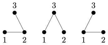
Here are the spanning trees for the $n=3$ case:
And here are a few of the $16$ spanning trees for the $n=4$ case:
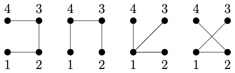
The answer for the first few $n$ are:
- $n=2: 1$
- $n=3: 3$
- $n=4: 16$
- $n=5: 125$
- $n=6: 1296$
You may have noticed that these numbers, especially for $n\geq 4$, are clean powers of integers.
If we write them out, we find
- $n=2: 1$
- $n=3: 3 = 3^1$
- $n=4: 16 = 4^2$
- $n=5: 125 = 5^3$
- $n=6: 1296 = 6^4$
It turns out that the pattern you're seeing here actually extends!
For every positive $n \geq 2$, the complete graph on $n$ vertices has $n^{n-2}$
spanning trees.
The proof to this theorem utilizes some counting arguments right at the edge of
what we've covered in this class. At this point you have the background to follow
and understand it, but it certainly has more ingenuity than any of the proofs
we've seen so far in class. That said, I think it's absolutely fascinating, and if
you agree then I encourage you to take more math and combinatorics courses!
The first thing we might try is a direct decision process, but it doesn't quite seem
to work out (I encourage you to try it!). Sure, our first decision might be to pick
a vertex ($n$ choices), but any natural next decision would involve making an edge,
which means picking a different vertex ($n-1$ choices). At this point, we've already
added a factor of $n-1$ that doesn't seem to be anywhere in the formula! Not to mention,
if we keep going down this path by adding edges, eventually it'll be unclear how many legal
decisions there are because the legality of a new edge depends on where the other edges are
placed, and that sounds like too many potential cycles to keep track of.
Instead, we'll do something really clever: we'll select a related set that's easier for us to count, and use
the relationship between the sets to figure out the size of the set we're interested in. (Problem-solving tip:
if you don't know how to solve a problem, try relating it to a problem you do know how to solve!)
In this case, let's consider the set of rooted, directed spanning trees.
I don't want to get too bogged down in the definitions, so you can think of it as picking a vertex on a non-directed
spanning tree to be the root, and turning each edge on the tree into an arrow that points outwards from the root.
The image below has some examples.
If this makes sense to you, feel free to skip ahead to the proof. If the definitions would help, here they are:
On a directed graph $G=(V, E)$, every edge $e=(v_i, v_j)$ is considered to
start at $v_i$ and end at $v_j$. In that sense, the edges can be thought of as arrows rather than lines,
and represent a one-way relationship from the start to the end.
For example, we might use a directed graph for a map with only one-way streets, or to model followings
on a social media platform where following isn't necessarily mutual.
On a directed graph $G=(V, E)$, a subgraph $G'=(V', E')$ is a rooted, directed tree if there is
some root vertex $r \in V'$ with the following property: for every vertex $v \in V'$, there is exactly one path
along $E'$ that starts at $r$ and ends at $v$.
You may notice that this is called a tree for good reason: if you remove the directionality of the subgraph,
it must be a tree as we've defined before. After all, it is connected (you can get to anywhere from $r$), and there are no cycles (or else
there would be two paths from $r$ to some $v$; see Theorem 10.16). A rooted, directed tree is just
a tree with a root and arrows flowing outwards from the root.
A rooted, directed spanning tree for a directed graph $G$ is, as the name suggests, a subgraph that is a
rooted, directed tree and is spanning.
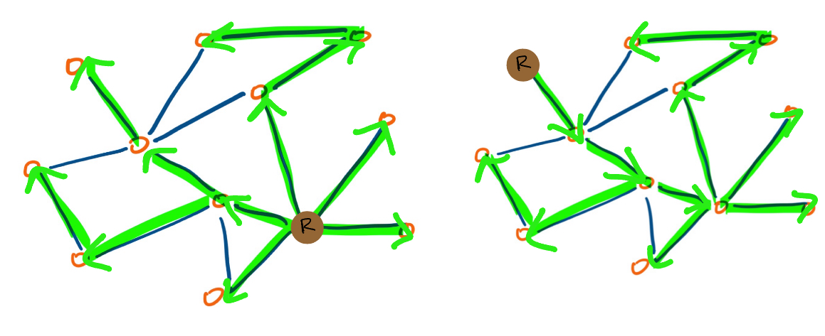
Here, are two different rooted directed spanning trees for the spanning tree we showed above. Notice how there's one root
and all the edges point outwards from the root.
With this related structure in mind, let's get to the proof of Cayley's Formula!
We are looking for the number of spanning trees of a complete
graph. As we mentioned earlier, a direct counting of
the number of spanning trees doesn't seem like it'll work, so instead we'll try to count the number of
rooted, directed spanning trees.
Method One. First, let's consider the decision process of constructing our rooted directed spanning tree
one directed edge at a time. At a glance, our decision process is:
- Select a directed edge to place on the tree.
- Select another directed edge to add that doesn't make it impossible to create a tree.
- Repeat step 2 until you've added $n-1$ edges (where $n=|V|$).
Computing the number of possibilities for step 1 is easy enough: there are $n$ choices for the start
of the edge and $n-1$ vertices for it to end at, so $n(n-1)$ possibilities. Let's think carefully about
step 2 now. We need to select a starting vertex and an ending vertex for step 2. As such, we need to
consider the following:
- What are the restrictions for the starting vertex?
- What are the restrictions for the ending vertex?
To think about this, let's say we've created some subset of the spanning tree. So
far, we've selected the following edges:
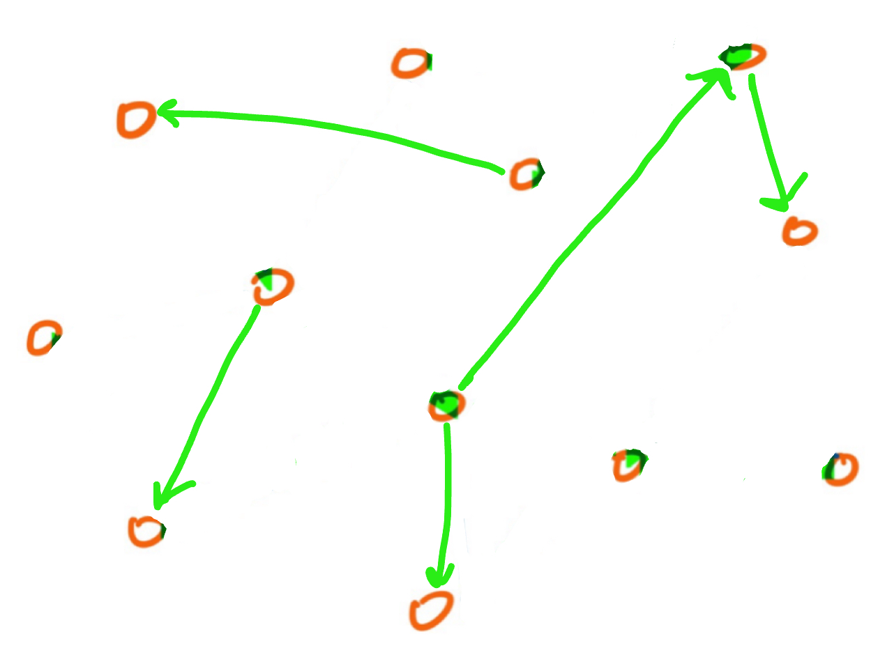
If we're at this point in the process, which vertices can we select to be the starting vertex?
In fact, any of them will be fine: a node on a tree can have more than one leaf, and no node
can not have leaves, so there are no restrictions for adding any arrows pointing away from a node.
On the other hand, can every vertex be an ending vertex? Not quite. Each vertex can be the start
for any number of edges, but can only be the end point for one edge. After all, if there are some
$v_1$ and $v_2$ that both point to $w$, then when the tree is completed the root will have paths
to both $v_1$ and $v_2$, which means it has two paths to $w$, so it's no longer a tree.
With this in mind, how many choices are there for the ending vertex? Let's say we've chosen our starting
vertex $v$. Each vertex can only be the ending vertex once, so after $i$ edges have been placed there are only $n-i$ possibilities remaining
for ending vertices. Furthermore, of there $n-i$ possibilities, either $v$ is among them, or an unchosen
vertex that leads to $v$ is among them. In either case, that possibility can not be selected (or else there'd be
a cycle), leaving us with $n-i-1$ total possibilities for end vertex.
So we've resolved our questions:
- What are the restrictions for the starting vertex? There are none -- any vertex
can be selected as a starting vertex for a new edge. Thus, we can select any of the $n$
vertices.
- What are the restrictions for the ending vertex? It can't be a vertex that has been chosen
previously to be an ending vertex, or one that leads to the starting vertex. Thus, there are
$n-i-1$ possibilities for the $i$th edge being placed.
That tells us that there are $n(n-i-1)$ ways to place the $i$th edge of this directed rooted
spanning tree. In total, our decision process tells us to select $n-1$ edges in total, so the number
of ways to do this is
$$(n)(n-1) \cdot (n)(n-2) \cdot \ldots \cdot (n)(1) = n^{n-1}\cdot (n-1)! $$
ways to construct this directed rooted spanning tree.
However, we've overcounted here! We gave an ordering to the edges of the tree, but the spanning tree does
not care what order the edges were placed in. In other words, the same tree could have been made if the edges
were selected in any other order. There are $n-1$ edges, for a total of $(n-1)!$ different orders in which the
edges could have been placed, so our final answer is that there are $n^{n-1}$ total directed rooted spanning trees.
Method Two. Here's a different decision process that we could follow to make a directed
rooted spanning tree:
- Select an undirected spanning tree on the graph.
- Select a vertex to be the root.
Once we've selected a root, the other edges only have one possible direction. Thus, this is all
we need to construct a directed rooted spanning tree! Remember that we don't actually know how many
different undirected spanning trees there are, but we can call that number $S_n$. In that case, by
this decision process, there are $S_n \cdot n$ different ways to construct a directed rooted spanning tree.
Bringing it together. You may be seeing where this is going. By method one, we found that there
are $n^{n-1}$ different directed rooted spanning trees. By method two, we found that there are $S_n \cdot n$
directed rooted spanning trees, where $S_n$ is the number of (undirected) spanning trees. By a little algebra,
we find that $S_n = n^{n-2}$, as desired.
Anyway, I think this proof is incredible: it combines combinatorial proofs from Unit 2 with the graph
theory we've done this unit, all with a neat twist of using a slightly easier problem to solve a more
difficult one. In all, I hope that through this class you gained the skills necessary to understand,
evaluate, and appreciate this proof, and that you take those skills and apply them to the problem-solving
and verification tasks that will face you for the years to come.